Dashboard as Code: Grafana
- GeekGuy
- Dec 13, 2021
- 11 min read
Updated: Jun 22, 2023
We faced the task of setting up monitoring for a client project. We solved that problem with grafonnet, a library that allows writing Grafana dashboards in a language called Jsonnet. This library saved us a lot of trouble.
The story is divided into two parts. In the first part, I’ll expand on how we got started with grafonnet. I’ll share why we chose this tool and what problems we solved with it. The second part is a tutorial on writing a simple Prometheus dashboard with grafonnet. Some situations described in the first part of the article may look familiar to you. In this case, the second part will help you take your first steps towards solving those problems.
1. Parenthetical remarks
1.1. How I met grafonnet
It all started with a problem, as usual.
At the end of 2019, our team was deploying two cache microservices into production. One of the items on our checklist was a configured monitoring system with incident alerts. The client already had a full-stack infrastructure: Telegraf, InfluxDB, and Grafana. After we’ve set up standard metrics and integrated Tarantool with the local systems, we had to represent tens of thousands of values in the form of production-ready graphs. I was tasked to find a solution.
Most people on our team had started working with Tarantool about a year before the events. Though we were quite experienced in the realm of development, monitoring was terra incognita for us. New metrics and changes in the existing ones were appearing several times a week. We were developing the Grafana dashboard iteratively — adding, deleting, and replacing panels. Each iteration began with a “creative” process, which boiled down to altering four dashboards instead of a single one. Providing an opportunity to monitor metrics for two different zones was one of the initial objectives. There were two possible solutions. Grafana requests can contain dynamic variables, such as values from the metrics database or arrays of constants. Variables let you easily transform a zone A dashboard into a zone B dashboard. Unfortunately, this convenient mechanism conflicts with alerts, which are no less useful. A panel’s alerting queries cannot contain variables. For this reason, we decided to support two static dashboards for every project.
We also wanted to optimize our routine tasks. In the beginning, the only difference between the two dashboards was their static query fields, so we initially used Ctrl+H to solve the problem.
Grafana can export dashboards as JSON. After making changes to one of the dashboards, we downloaded it and used a text editor to replace variable values in the queries. For more complex replacements, we wrote a Python script that read the transformation rules from a YAML file. As the caches had separate mechanisms for Oracle replication and cold data upload, the dashboards became utterly different at some point — with different sets of graphs. Deleting a panel with a script is easy, but adding a panel in this way is much more complicated. One day we saw that the dashboard transformation script was becoming a tool to generate new dashboards. Evidently, someone else must have already found a solution to that problem. Among such solutions were publicly available projects like Weaveworks grafanalib, Uber Grafana dashboard generator, Showmax Grafana dashboard generator, grafyaml, and grafonnet. Besides, out-of-the-box Grafana allowed creating dashboards with JavaScript. We also considered developing our custom dashboard generator. Ultimately, our situation helped us narrow our choice down to grafonnet, the only tool that could send queries to InfluxDB.
1.2. Beginnings
Grafonnet is a Grafana open-source project for writing dashboards as code (see GitHub page). It includes templates for various Grafana panel and query types, variables, and methods to bring that all together in a dashboard. One of the main advantages of grafonnet is that it uses Jsonnet — a concise and straightforward language. As you usually process expanded JSON objects that support hidden and function fields, you can manually finalize the result at any stage without altering the code itself.
Nevertheless, what we started with was customizing the source code of grafonnet. Table and stat panels lacked some elements introduced in Grafana v6, and there was no template for the Status Panel custom extension. Despite the support for InfluxDB requests, grafonnet didn’t allow using blocks to specify requests, only working with raw InfluxQL. To add a panel to a dashboard, you had to manually recalculate the coordinates of all the panels below. This problem was also solved with a Jsonnet script, which embedded itself into the dashboard during panel build and found the right place for each panel based on size. Our key solutions were passed to grafonnet via pull requests and are now available to all users.
After we transferred the aforementioned projects to grafonnet, our client commissioned us another project — a universal dashboard for all their Tarantool-based services. Using the code of the first version, we managed to throw together a universal template that also supported extensions. Anyone could create custom, project-specific graphs and add them to their dashboard during the build. Raw JSON would require much more work.
1.3. Gaining ground
When the project reached a certain level of readiness, we decided to create a derivative — an open-source dashboard for the standard Tarantool Cartridge application. It can be found among Grafana official and community dashboards: version for InfluxDB, version for Prometheus. The source code is available on GitHub.

Initially, we were only going to develop a version for InfluxDB, as we had both expertise and some work already done. However, our metrics package supports metric output in the Prometheus format, which is popular among users. This led to us developing a version for Prometheus. Visualization in panels is query-independent, which allows efficiently reusing code. Moreover, working with ready-made templates saves a lot of trouble when you have to add many similar panels at once.
2. Grafonnet in practice
2.1. Introduction to Jsonnet
We’ll need Jsonnet v0.16.0. The implementation used in Tarantool projects is Go-based (see GitHub page).
First, let’s discuss the key points of using Jsonnet. The official project website has a detailed tutorial and a description of the standard function library. A Jsonnet script returns valid JSON — a string, a boolean, a number, null, an array, or an object (dictionary). Let’s write a basic script:
# script1.jsonnet
{
    field: 1 + 2
}
Use the following command to execute the script:
jsonnet script1.jsonnetYou will see the result in the console:
{
   "field": 3
}
To save the output to a file, pass the -o flag:
jsonnet script1.jsonnet -o result.jsonSometimes it’s convenient to put the result in the clipboard. The xclip utility lets you do this:
jsonnet script1.jsonnet | xclip -selection clipboardThere are two types of Jsonnet scripts — .libsonnet and .jsonnet. While .libsonnet scripts produce intermediary structures, .jsonnet scripts are used to generate end results. Apart from the JSON type, Jsonnet supports functions. Besides, Jsonnet objects can contain hidden fields, assigned with the “::” operator. Let’s create a math utilities library:
# math.libsonnet
{
    sum(a, b): a + b
}
Files can be connected with import. We’ll now use our library in a script:
# script2.jsonnet
local math = import 'math.libsonnet';{
    field: math.sum(1, 2)
}
The result will be the object that we’ve already seen above. You can also have local variables in the script:
# script3.jsonnet
local math = import 'math.libsonnet';
local value = math.sum(1, 2);{
    field: value
}
Local variables can also be declared within objects:
# script4.jsonnet
local math = import 'math.libsonnet';{
    local value = math.sum(1, 2),
    field: value
}
These variables are ignored by the import construct and during end result calculation.
jsonnet script4.jsonnet{
   "field": 3
}
2.2. Installing grafonnet
First, install dependencies with jsonnet-bundler. Then, initialize your project with the following command:
jb initA file named jsonnetfile.json will be created in your project. Add the grafonnet repository to it:
{
  "version": 1,
  "dependencies": [
    {
      "source": {
        "git": {
          "remote": "https://github.com/grafana/grafonnet-lib",
          "subdir": "grafonnet"
        }
      },
      "version": "master"
    }
  ],
  "legacyImports": true
}
Now run the following command:
jb installJsonnet-bundler will download the repositories and register the commits in the lock file. This is convenient if you’re adding a dependency from a specific branch:
{
  "version": 1,
  "dependencies": [
    {
      "source": {
        "git": {
          "remote": "https://github.com/grafana/grafonnet-lib.git",
          "subdir": "grafonnet"
        }
      },
      "version": "3082bfca110166cd69533fa3c0875fdb1b68c329",
      "sum": "4/sUV0Kk+o8I+wlYxL9R6EPhL/NiLfYHk+NXlU64RUk="
    }
  ],
  "legacyImports": false
}
On all further calls, jb install will access the lock file. I recommend using the version specified above for this tutorial.
2.3. Creating a dashboard
Generally, the dashboard has the following structure:

I use Grafana v6 in my tutorial. Although the dashboard works with later versions of Grafana, we won’t be using their new features.
2.3.1. Empty dashboard
First, let’s create an empty dashboard:
# dashboard.jsonnet
local grafana = import 'grafonnet/grafana.libsonnet';grafana.dashboard.new(
    title='My dashboard'
)
To compile the dashboard, run the following:
jsonnet -J ./vendor dashboard.jsonnet -o dashboard.jsonThe -J flag allows connecting external libraries. In our case, we’ll use the ./vendor directory that contains the dependencies installed by jsonnet-bundler.
2.3.2. Practice Docker cluster
I created a Docker cluster where you can practice. It contains a simple Tarantool application, Prometheus, and Grafana, and it is available as a GitHub repo. Clone it and run the command below (requires docker-compose):
docker-compose upAfter launch, Grafana will be available at localhost:3000.
2.3.3. Importing the dashboard
To upload your dashboard from JSON, use the import function in the Grafana sidebar.
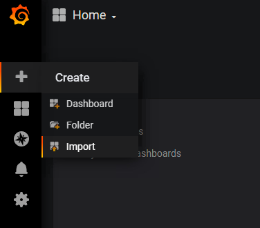
Upload a file or paste JSON from clipboard. At the next step, enter the name of your dashboard and choose a directory for it.

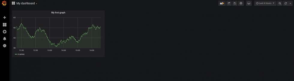
The result will be an empty dashboard:

2.3.4. Adding panels
Let’s add a graph panel to our dashboard:
local grafana = import 'grafonnet/grafana.libsonnet';grafana.dashboard.new(
    title='My dashboard',
    # allow the user to make changes in Grafana
    editable=true,
    # avoid issues associated with importing multiple versions in Grafana
    schemaVersion=21,
).addPanel(
    grafana.graphPanel.new(
        title='My first graph',
        # demonstration data
        datasource='-- Grafana --'
    ),
    # panel position and size
    gridPos = { h: 8, w: 8, x: 0, y: 0 }
)
Now let’s build the dashboard:
jsonnet -J ./vendor dashboard.jsonnet -o dashboard.jsonYou can overwrite an existing dashboard or choose a different name on import.
Let’s focus on gridPos. The size and position of every panel are described with grid coordinates. The dashboard width is 24 units. This means that a _row_ panel has a size of 24x1. When you add a panel, it has a size of 12x9 by default.
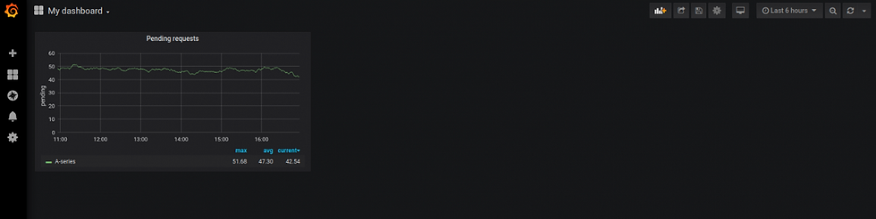
2.3.5. Visualization settings
Panels are created as a result of function calls. To set up metric visualization in the panels, we have to change the parameters of these functions.
local grafana = import 'grafonnet/grafana.libsonnet';grafana.dashboard.new(
    title='My dashboard',
    editable=true,
    schemaVersion=21,
).addPanel(
    grafana.graphPanel.new(
        title='Pending requests',
        datasource='-- Grafana --',
        # Lowest displayed value
        min=0,
        # Left y-axis legend
        labelY1='pending',
        # Color intensity of the area under the graph
        fill=0,
        # Number of decimal places in values
        decimals=2,
        # Number of decimal places in left y-axis values
        decimalsY1=0,
        # Sort the values in decreasing order
        sort='decreasing',
        # Present the legend as a table
        legend_alignAsTable=true,
        # Display values in the legend
        legend_values=true,
        # Display the average value in the legend
        legend_avg=true,
        # Display the current value in the legend
        legend_current=true,
        # Display the maximum in the legend
        legend_max=true,
        # Sort by current value
        legend_sort='current',
        # Sort in descending order
        legend_sortDesc=true,
    ),
    gridPos = { h: 8, w: 8, x: 0, y: 0 }
)
All the panel parameters are described in grafonnet sources. In particular, you can find graph options in vendor/grafonnet/graph_panel.libsonnet.
2.3.6. Forming a query to Prometheus
Let’s visualize the server_pending_requests metric from our test application.
local grafana = import 'grafonnet/grafana.libsonnet';

 grafana.dashboard.new(
     title='My dashboard',
     editable=true,
     schemaVersion=21,
     # Display metrics over the last 30 minutes
     time_from='now-30m'
 ).addPanel(
     grafana.graphPanel.new(
         title='Pending requests',
         # Direct queries to the `Prometheus` data source
         datasource='Prometheus',
         min=0,
         labelY1='pending',
         fill=0,
         decimals=2,
         decimalsY1=0,
         sort='decreasing',
         legend_alignAsTable=true,
         legend_values=true,
         legend_avg=true,
         legend_current=true,
         legend_max=true,
         legend_sort='current',
         legend_sortDesc=true,
     ).addTarget(
         grafana.prometheus.target(
             # Query 'server_pending_requests' from datasource
             expr='server_pending_requests',
             # Label query results as 'alias'
             # (corresponds to specific instances in the application cluster)
             legendFormat='{{alias}}',
         )
     ),
     gridPos = { h: 8, w: 8, x: 0, y: 0 }
 )
The _addTarget()_ method can be called several times.
2.3.7. Import variables
A JSON dashboard can involve variables defined on import. In this way, we can configure datasource, the source of metrics for your dashboard.
local grafana = import 'grafonnet/grafana.libsonnet';grafana.dashboard.new(
    title='My dashboard',
    editable=true,
    schemaVersion=21,
    time_from='now-30m'
).addInput( # add an import variable
    # Variable name to be used in the dashboard code
    name='DS_PROMETHEUS',
    # Variable name to be displayed on the import screen
    label='Prometheus',
    # This variable defines the data source
    type='datasource',
    # Data will be received from the Prometheus plugin
    pluginId='prometheus',
    pluginName='Prometheus',
    # Variable description to be displayed on the import screen
    description='Prometheus metrics bank'
).addPanel(
    grafana.graphPanel.new(
        title='Pending requests',
        # Use the variable value as a data source
        datasource='${DS_PROMETHEUS}',
        min=0,
        labelY1='pending',
        fill=0,
        decimals=2,
        decimalsY1=0,
        sort='decreasing',
        legend_alignAsTable=true,
        legend_values=true,
        legend_avg=true,
        legend_current=true,
        legend_max=true,
        legend_sort='current',
        legend_sortDesc=true,
    ).addTarget(
        grafana.prometheus.target(
            expr='server_pending_requests',
            legendFormat='{{alias}}',
        )
    ),
    gridPos = { h: 8, w: 8, x: 0, y: 0 }
)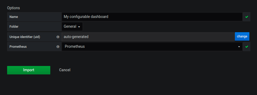
Now you can select a data source from the drop-down list automatically created by Grafana.
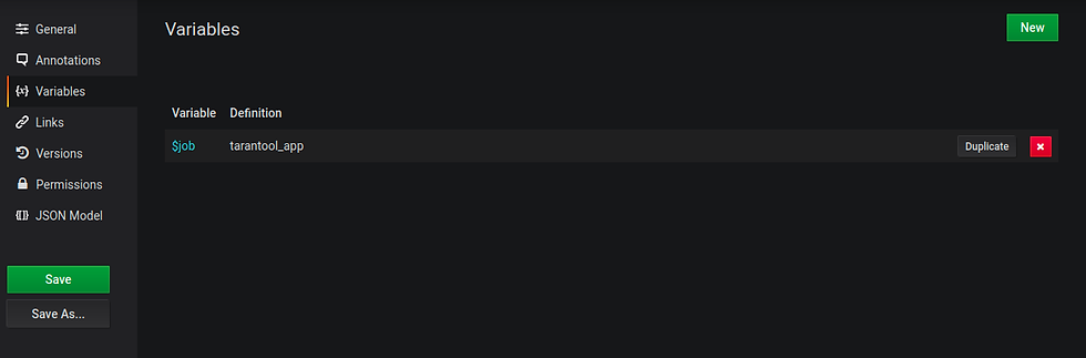
2.3.8. Dynamic variables
There are two types of variables in Grafana: __inputs and templating. While __inputs are defined on import and become “frozen” in the dashboard, templating variables can be changed during operations. Working with an __inputs variable involves replacing ${VAR_NAME} text strings with a custom value. However, you can’t do this in data source queries — you use templating variables instead. One of the methods to divide data coming from different applications is to use different Prometheus jobs to collect them. You can register the job in your query and configure it on import.
 local grafana = import 'grafonnet/grafana.libsonnet';

 grafana.dashboard.new(
     title='My dashboard',
     editable=true,
     schemaVersion=21,
     time_from='now-30m'
 ).addInput(
     name='DS_PROMETHEUS',
     label='Prometheus',
     type='datasource',
     pluginId='prometheus',
     pluginName='Prometheus',
     description='Prometheus metrics bank'
 ).addInput( # string constant to be filled in on import
     name='PROMETHEUS_JOB',
     label='Job',
     type='constant',
     pluginId=null,
     pluginName=null,
     description='Prometheus Tarantool metrics job'
 ).addTemplate(
     grafana.template.custom( # dynamic variable
         # Variable name to be used in the dashboard code
         name='job',
         # Initial dynamic variable value is derived from the import variable
         query='${PROMETHEUS_JOB}',
         current='${PROMETHEUS_JOB}',
         # Don't display the variable on the panel screen
         hide='variable',
         # Variable name in the UI
         label='Prometheus job',
     )
 ).addPanel(
     grafana.graphPanel.new(
         title='Pending requests',
         datasource='${DS_PROMETHEUS}',
         min=0,
         labelY1='pending',
         fill=0,
         decimals=2,
         decimalsY1=0,
         sort='decreasing',
         legend_alignAsTable=true,
         legend_values=true,
         legend_avg=true,
         legend_current=true,
         legend_max=true,
         legend_sort='current',
         legend_sortDesc=true,
     ).addTarget(
         grafana.prometheus.target(
             # Use the variable in our request
             expr='server_pending_requests{job=~"$job"}',
             legendFormat='{{alias}}',
         )
     ),
     gridPos = { h: 8, w: 8, x: 0, y: 0 }
 )
In our practice Docker cluster, job has the value of tarantool_app.
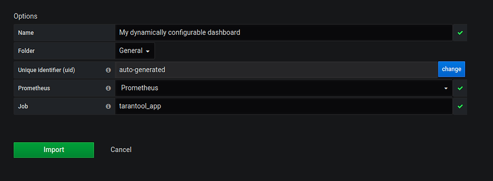
We applied two-level parametrization: job is regulated by a templating variable, while that variable’s initial value is defined on import through an __inputs variable. If you specified the wrong job during import, you can change it via your dashboard parameters.
2.3.9. Using functions
Let’s add one more panel, which will display the number or requests per second.
local grafana = import 'grafonnet/grafana.libsonnet';grafana.dashboard.new(
    title='My dashboard',
    editable=true,
    schemaVersion=21,
    time_from='now-30m'
).addInput(
    name='DS_PROMETHEUS',
    label='Prometheus',
    type='datasource',
    pluginId='prometheus',
    pluginName='Prometheus',
    description='Prometheus metrics bank'
).addInput(
    name='PROMETHEUS_JOB',
    label='Job',
    type='constant',
    pluginId=null,
    pluginName=null,
    description='Prometheus Tarantool metrics job'
).addInput( # initial rate_time_range value
    name='PROMETHEUS_RATE_TIME_RANGE',
    label='Rate time range',
    type='constant',
    value='2m',
    description='Time range for computing rps graphs with rate(). Should be two times the scrape interval at least.'
).addTemplate(
    grafana.template.custom(
        name='job',
        query='${PROMETHEUS_JOB}',
        current='${PROMETHEUS_JOB}',
        hide='variable',
        label='Prometheus job',
    )
).addTemplate( # dynamic variable to be used in the query
    grafana.template.custom(
        name='rate_time_range',
        query='${PROMETHEUS_RATE_TIME_RANGE}',
        current='${PROMETHEUS_RATE_TIME_RANGE}',
        hide='variable',
        label='rate() time range',
    )
).addPanel(
    grafana.graphPanel.new(
        title='Pending requests',
        datasource='${DS_PROMETHEUS}',
        min=0,
        labelY1='pending',
        fill=0,
        decimals=2,
        decimalsY1=0,
        sort='decreasing',
        legend_alignAsTable=true,
        legend_values=true,
        legend_avg=true,
        legend_current=true,
        legend_max=true,
        legend_sort='current',
        legend_sortDesc=true,
    ).addTarget(
        grafana.prometheus.target(
            expr='server_pending_requests{job=~"$job"}',
            legendFormat='{{alias}}',
        )
    ),
    gridPos = { h: 8, w: 8, x: 0, y: 0 }
).addPanel( # server load graph
    grafana.graphPanel.new(
        title='Server load',
        datasource='${DS_PROMETHEUS}',
        min=0,
        labelY1='rps',
        fill=0,
        decimals=2,
        decimalsY1=0,
        sort='decreasing',
        legend_alignAsTable=true,
        legend_avg=true,
        legend_current=true,
        legend_max=true,
        legend_values=true,
        legend_sort='current',
        legend_sortDesc=true,
        legend_rightSide=true,
    ).addTarget(
        grafana.prometheus.target(
            # Compute changes using the data from the rate_time_range period
            expr='rate(server_requests_process_count{job=~"$job"}[$rate_time_range])',
            legendFormat='{{alias}}',
        )
    ),
    # Put the panel on the right of the first one
    gridPos = { h: 8, w: 16, x: 9, y: 0 }
)
The import variable can be initialized in the code.

As a result, we have a dashboard with two panels:

Let’s clean up our code by moving the graph template to a function:
local grafana = import 'grafonnet/grafana.libsonnet';local myGraphPanel(
  title=null,
  labelY1=null,
  legend_rightSide=false # default value
) = grafana.graphPanel.new(
    title=title,
    datasource='${DS_PROMETHEUS}',
    min=0,
    labelY1=labelY1,
    fill=0,
    decimals=2,
    decimalsY1=0,
    sort='decreasing',
    legend_alignAsTable=true,
    legend_values=true,
    legend_avg=true,
    legend_current=true,
    legend_max=true,
    legend_sort='current',
    legend_sortDesc=true,
    legend_rightSide=legend_rightSide
);grafana.dashboard.new(
    title='My dashboard',
    editable=true,
    schemaVersion=21,
    time_from='now-30m'
).addInput(
    name='DS_PROMETHEUS',
    label='Prometheus',
    type='datasource',
    pluginId='prometheus',
    pluginName='Prometheus',
    description='Prometheus metrics bank'
).addInput(
    name='PROMETHEUS_JOB',
    label='Job',
    type='constant',
    pluginId=null,
    pluginName=null,
    description='Prometheus Tarantool metrics job'
).addInput(
    name='PROMETHEUS_RATE_TIME_RANGE',
    label='Rate time range',
    type='constant',
    value='2m',
    description='Time range for computing rps graphs with rate(). Should be two times the scrape interval at least.'
).addTemplate(
    grafana.template.custom(
        name='job',
        query='${PROMETHEUS_JOB}',
        current='${PROMETHEUS_JOB}',
        hide='variable',
        label='Prometheus job',
    )
).addTemplate(
    grafana.template.custom(
        name='rate_time_range',
        query='${PROMETHEUS_RATE_TIME_RANGE}',
        current='${PROMETHEUS_RATE_TIME_RANGE}',
        hide='variable',
        label='rate() time range',
    )
).addPanel(
    myGraphPanel(
        title='Pending requests',
        labelY1='pending'
    ).addTarget(
        grafana.prometheus.target(
            expr='server_pending_requests{job=~"$job"}',
            legendFormat='{{alias}}',
        )
    ),
    gridPos = { h: 8, w: 8, x: 0, y: 0 }
).addPanel(
    myGraphPanel(
        title='Server load',
        labelY1='rps',
        legend_rightSide=true,
    ).addTarget(
        grafana.prometheus.target(
            expr='rate(server_requests_process_count{job=~"$job"}[$rate_time_range])',
            legendFormat='{{alias}}',
        )
    ),
    gridPos = { h: 8, w: 16, x: 9, y: 0 }
)
It may be convenient to move the template to a separate file. Try doing this on your own as an exercise. To learn about connecting external files, see the section on Jsonnet above.
3. Final words
Grafana dashboards as code are not a silver bullet. However, there are cases where this approach has proven effective. It presents vast opportunities for static configuration, has a convenient versioning mechanism, and its results can be reused between projects. This is why I wanted to share with you how to create dashboards with grafonnet. The final version of my tutorial lacks a few specific points. I have enough material for a whole second article on those points. Please leave feedback if you want to see it published! To sum it up, below are a few useful links. The grafonnet repository contains grafonnet source code and documentation, as well as several examples of how to use templates. By the way, several PRs of mine are still awaiting review, so please support them if you find them interesting. The source code of the Tarantool dashboard is written in grafonnet. The code snippets in my tutorial and the Docker cluster are the results of my work and the work of my colleagues on this project. If you have any questions on the Tarantool dashboard or its extensions, ask them in GitHub Issues or in our Telegram chat. Tarantool can be downloaded on the official website.

Comments